Acknowledgement: Thanks again to Arthur Eckstein whose efforts in checking, adhering to and verifying this guide have once again proved invaluable.

AutolevellerAE was designed as a tool for measuring the minute changes in height throughout your work-piece so that when it comes to milling/etching we can use those measurements to adjust the Z height throughout the mill and thus achieve a more even and levelled result. This guide will use the latest current member version (0.9.2 at time of writing) when examples and screenshots are needed, however the guide can be followed in part with the free AutolevellerAE download.

Note that there are many features in AutolevellerAE which we will brush past in this guide (such as custom controller options and segment length settings) because the aim here is to get you producing levelled mills as quickly as possible and not to provide a detailed breakdown of every part of AE. The additional options will be described and explained in a full guide to AutolevellerAE.

1             Installation and setup

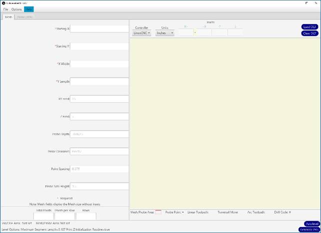
AE does not require installing as most other programs on your system. AE is a single, selfcontained file which you can just download, “double-click” and run (see figure 1).

To get to this point, you will first need Java 8 installed which can be downloaded from https://java.com/download/

You can check which version of java you have installed by typing java -version at the console/command prompt. This is what happens when I type it at my command prompt:

--> java -version 

java version "1.8.0_121"
Java(TM) SE Runtime Environment (build 1.8.0_121-b13)
Java HotSpot(TM) 64-Bit Server VM (build 25.121-b13, mixed mode)

You can see that I have update 121 of Java 8 installed but anything above update 80 is fine. At time of writing update 144 is the latest update to Java 8.

Most machines will have Java installed anyway so you might not need to install Java at all.

To download AE, go to the download page for this site.

You may see that there is a .exe download as well as a .jar, downloading and “double– clicking” either will start AE. Download the file of your choice and save to a location you can remember. Note there is no “installation” procedure so a handy location on your Windows machine might be something like C:\Autoleveller\. At this point users could also create a shortcut to place on your desktop for easy implementation of the program. The .exe file is just a wrapper around the .jar and is exactly the same file in all other respects. The .exe file is provided because it is probably more familiar to Windows users but either file should work fine on Windows.

If you are not on a Windows system, you must use the .jar file and type java -jar AutolevellerAE-0.9.2.jar at your console to start. (or whatever the .jar filename is) Whichever file type you use, you should now see something similar to figure 1.

2             Generating a Mesh/Probe area

The area you will be probing i.e the Mesh, first needs to be defined, and there are 2 ways to do this.

2.1           Manually defining the Mesh

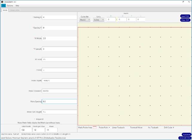
We can manually enter the Mesh values for the area we want to probe as in figure 2.

As soon as you enter the first 4 values (X, Y, X width and Y length) you should see the red outline of the mesh/probe area appear. As you can see from the figure, I have specified a probe area 3.5” wide by 3” high. The coloured dots within this area mark the relative locations of the probe points and you can see the total points displayed in the bottom left.

You can change the probe spacing value if you want to increase or reduce the number of probe points but you need to strike a balance between lots of points to increase the accuracy of your mill and few points to reduce probing time. The number of points will depend on the size of your job so it might take some experimentation before you find a probe spacing value you are happy with. As a rule of thumb I try for a probe spacing of 10mm or about 0.4”. This depends on the size of the area being covered though.

2.2           Automatically defining the Mesh

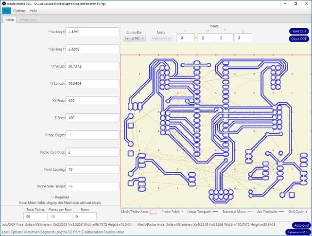
A far more common and easier approach is to load a GCode file and have AE calculate the correct size for the mesh automatically, as shown in figure 3.

As soon as I load the original GCode file (OGF), the mesh is generated and the red box appears round the job. I can of course change any of the Mesh settings as before. Here I have changed the probe spacing to 10mm and have set the insets to -2mm which makes the probe area 2mm larger in all directions.

3             Probing Preparations

Now that we have our Mesh/probing area defined, we need to ensure our probe is ready and working at our CNC machine. The simplest and most common way to do this is with an electrical probe, this way you can use the same tool for probing as you do for the milling, and avoids swapping tools around. Setting up an electrical probe is described in the probe guide. Of course an electrical probe is not helpful if you are probing wood or plastic, for this you can cover the surface in a thin piece of foil first, or use a non-electrical probe.

4             Standard Levelling

As long as you have an OGF and Mesh defined as in figure 3 you can just click on ‘Autolevel’ and a single GCode file will be produced containing everything needed to etch your job, i.e.

the probing stage, calculations and GCode modifications.

In this GCode file, you will see a series of statements at the top, like this:

...
G0 Z2
G1 X73.2948 Y144.79504 F600
G31 Z-1 F100
#717=#2002
G0 Z2
G1 X83.3959 Y144.79504 F600
G31 Z-1 F100 #718=#2002 
...

These probe each point as shown in your Mesh image earlier and record each Z value in a parameter like #717 and #718 etc. Now we can use these recorded values to calculate the most appropriate Z value during the etching process.

Later in the file you will see that your original GCode has been re-printed but with several calculations and modifications to Z. You will see many lines like this:

...
#102=[#605+0.97963*#590-0.97963*#605]
#101=[#606+0.97963*#591-0.97963*#606]
#100=[#102+0.99800*#101-0.99800*#102] 
G01 X12.6680 Y63.9027Z[#100+-0.2]
#102=[#605+0.97948*#590-0.97948*#605]
#101=[#606+0.97948*#591-0.97948*#606]
#100=[#102+0.99735*#101-0.99735*#102] 
G01 X12.6614 Y63.9042Z[#100+-0.2] 
...

So, for each etching line there are 3 lines of calculations to work out what the value of Z should be. Because we don’t know what the probed point values will be until the file is run on your CNC machine the calculations are performed at the moment they are needed rather than being pre-calculated as with the 2-stage levelling approach.

5             2-stage Levelling

Rather than probing the work-piece, storing the probed values in variables then calculating Z and levelling “on the fly” all in 1 GCode file, we can separate the 2 main processes into 2 distinct stages. The probing stage records probe values to a log file rather than to parameters. In the levelling stage we can then take this log file and load it into AE. Because the probed values are known and recorded in the log file, AE can perform all calculations “in-house” and not have to write the maths to the GCode output.

5.1           Stage 1: Probing

So, we still need a Mesh for this part, which we created in section 2, but, instead of clicking ‘Autolevel’, we click ‘Generate PFG’ (Probe File Generator) and save the file somewhere. This GCode file is essentially just the probing part of a standard Autolevelled file, but instead of recording the probed values to parameters as before we are now writing them to a separate file, which is called the Raw Probe File (RPF). What we want to do is take this RPF and apply it directly to our original GCode so that we can do all calculations and level Z from the real probed values in the RPF and not need to write any maths to the Autolevelled GCode as before.

RPF

Each time the probe makes contact with the surface it records the probed value to the RPF, which is just a plain text file comprising an ordered list of the point values in question. If you are using Mach3 you will be asked where to save it when you run the PFG (you can name it anything you like). In LinuxCNC the RPF will be saved as ‘RawProbeLog.txt’ in the same folder as your .ini file. In TurboCNC, the file will be named Points.dat and will be located in the same directory as the system file.

For Mach3 the contents will look something like this:

...
3.89841,0.77490,0.00260
3.89841,1.16236,-0.00975
3.50857,1.16236,0.00386
3.11873,1.16236,0.00441
2.72888,1.16236,0.00472
...

In LinuxCNC the contents look something like this:

...
3.898400 0.774900 -0.003151 0.000000 0.000000 0.000000 0.000000 0.000000 0.000000
3.898400 1.162350 -0.007981 0.000000 0.000000 0.000000 0.000000 0.000000 0.000000
3.508560 1.162350 0.002096 0.000000 0.000000 0.000000 0.000000 0.000000 0.000000
3.118720 1.162350 0.003012 0.000000 0.000000 0.000000 0.000000 0.000000 0.000000
2.728880 1.162350 0.003262 0.000000 0.000000 0.000000 0.000000 0.000000 0.000000 
...

In TurboCNC something like this:

...
X -1.502394Y 1.241511Z 0.001093A 0.000000
X -1.878018Y 1.241511Z -0.001043A 0.000000
X -2.253592Y 1.241511Z -0.002484A 0.000000
X -2.629215Y 1.241511Z -0.003478A 0.000000
X -2.629215Y 1.655382Z -0.001888A 0.000000 
...

NOTE: For TurboCNC, you MUST delete the Points.dat file just before probing or it will contain extraneous data and will fail during subsequent use. Further this will not work in the original Autoleveller.

If you are experimenting with a custom controller you may have another format. Whatever controller you use, the first 3 numbers in each line will be parsed by AE as the X, Y and Z values. Any further numbers in the line will be ignored by AE. So you could even use a different style or write a program for GRBL to create your own RPF for example. As long as you adhere to this 3 distinct number format, AE will be able to read it.

One other restriction by AE is that all the Y values must be the same for all points within the same row for AE to consider them the same. Likewise, all X values must be the same for all values within the same the same column for AE to consider them the same. Otherwise AE will probably see that there is a different number of points in different rows and refuse to load the file. If you are struggling to get your X and Y values the same, try reducing the XY feedrate in the Mesh set-up. This should give your machine a better chance of stopping at the XY coordinate that its supposed to stop at during probing and not to overshoot its target.

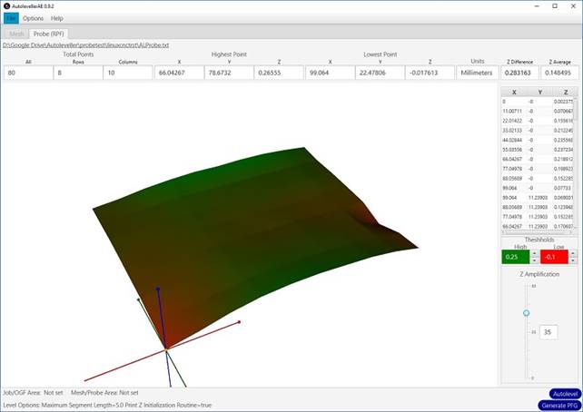
Assuming the RPF is valid, you can load it into AE (File → Raw Probe File) and it should open in the Probe tab which lets you view the area you just probed and spot any problems with it before using the file in levelling. See figure 4.

Here we have adjusted the threshold values for color and set the Z amplification to 35 to exaggerate the high and low points. The tab shows other useful statistics based on your RPF such as highest and lowest points, difference in highest and lowest Z values (effectively a measure of how flat the probed surface is), an average for Z as well as a table showing every probed point in the file.

5.2           Stage 2: Levelling

Once we have an OGF and an RPF loaded into AE, clicking ‘Autolevel’ will use the RPF to level and create the output rather than printing some calculations to the GCode file, i.e. the calculations are pre-empted by AE and not by your controller. Save the output as before except now the file should be much smaller without the maths in the GCode output. Separating the probing and levelling like this has a few advantages…

• We never need to perform the probing more than once unless the work-piece has moved or flipped etc.
• Can easily stop etching and resume the next day or re-start the etch from the beginning if you tool breaks of something, all without the need to re-probe.
• We can easily use one tool for probing and another for the milling/etching
• Can inspect and ‘debug’ the RPF before committing to levelling
• Easier to spot mistakes in the Z values of the levelled file, since these will be real numbers and not calculations
• Smaller file size